
To get cracking, we need some flow cytometry data (i.e., .fcs files).
A few FCS data files have been bundled with this python package.
To use these files, enter the following in your ipython terminal:
In [1]: import os, FlowCytometryTools;

In [2]: datadir = os.path.join(FlowCytometryTools.__path__[0], 'tests', 'data', 'Plate01');

In [3]: datafile = os.path.join(datadir, 'RFP_Well_A3.fcs');
Note
To analyze your own data, simply set the ‘datafile’ variable to the path of your .fcs file:
>>> datafile=r'C:\data\my_very_awesome_data.fcs'
** Windows Users **
Windows uses the backslash character (‘’) for paths. However, the backslash character is a special character in python that is used for formatting strings. In order to specify paths correctly, you must precede the path with the character ‘r’.
Good:
>>> datafile=r'C:\data\my_very_awesome_data.fcs'
Bad:
>>> datafile='C:\data\my_very_awesome_data.fcs'
Below is a brief description, for more information see FCMeasurement.
Once datadir and datafile have been defined, we can proceed to load the data:
In [4]: from FlowCytometryTools import FCMeasurement

In [5]: sample = FCMeasurement(ID='Test Sample', datafile=datafile)
Want to know which channels were measured? No problem.
In [6]: print sample.channel_names
('HDR-T', 'FSC-A', 'FSC-H', 'FSC-W', 'SSC-A', 'SSC-H', 'SSC-W', 'V2-A', 'V2-H', 'V2-W', 'Y2-A', 'Y2-H', 'Y2-W', 'B1-A', 'B1-H', 'B1-W')
In [7]: print sample.channels
                 $PnN  $PnB $PnG                  $PnE   $PnS    $PnR
Channel Number
1               HDR-T    32    1  [0.000000, 0.000000]  HDR-T  262144
2               FSC-A    32    1  [0.000000, 0.000000]  FSC-A  262144
3               FSC-H    32    1  [0.000000, 0.000000]  FSC-H  262144
4               FSC-W    32    1  [0.000000, 0.000000]  FSC-W  262144
5               SSC-A    32    1  [0.000000, 0.000000]  SSC-A  262144
6               SSC-H    32    1  [0.000000, 0.000000]  SSC-H  262144
7               SSC-W    32    1  [0.000000, 0.000000]  SSC-W  262144
8                V2-A    32    1  [0.000000, 0.000000]   V2-A  262144
9                V2-H    32    1  [0.000000, 0.000000]   V2-H  262144
10               V2-W    32    1  [0.000000, 0.000000]   V2-W  262144
11               Y2-A    32    1  [0.000000, 0.000000]   Y2-A  262144
12               Y2-H    32    1  [0.000000, 0.000000]   Y2-H  262144
13               Y2-W    32    1  [0.000000, 0.000000]   Y2-W  262144
14               B1-A    32    1  [0.000000, 0.000000]   B1-A  262144
15               B1-H    32    1  [0.000000, 0.000000]   B1-H  262144
16               B1-W    32    1  [0.000000, 0.000000]   B1-W  262144
In addition to the raw data, the FCS files contain “meta” information about the measurements, which may be useful for data analysis. You can access this information using the meta property, which will return to you a python dictionary. The meaning of the fields in meta data is explained in the FCS format specifications (google for the specification).
In [8]: print type(sample.meta)
<type 'dict'>

In [9]: print sample.meta.keys()
['$ETIM', '$ENDDATA', '$BYTEORD', '$SRC', '_channels_', '$SYS', '$PAR', '$ENDANALYSIS', '$CYT', '__header__', '$BTIM', '$OP', '$BEGINANALYSIS', '$BEGINDATA', '$ENDSTEXT', '$CYTSN', '$DATE', '$MODE', '$FIL', '$BEGINSTEXT', '$NEXTDATA', '$CELLS', '$TOT', '_channel_names_', '$DATATYPE']

In [10]: print sample.meta.['$SRC']
  File "<ipython-input-10-a745febfc7b2>", line 1
    print sample.meta.['$SRC']
                      ^
SyntaxError: invalid syntax
The data is accessible as a pandas.DataFrame.
In [11]: print type(sample.data)
<class 'pandas.core.frame.DataFrame'>

In [12]: print sample.data[['Y2-A', 'FSC-A']][:10]
          Y2-A        FSC-A
0   109.946274   459.962982
1  5554.108398  -267.174652
2    81.835281  -201.582336
3   -54.120304   291.259888
4   -10.542595  -397.168579
5    34.791252  -213.151566
6  6132.993164   -25.696339
7    33.034771    61.271519
8  6688.348633  1462.823608
9    14.344463   490.025482
If you do not know how to work with DataFrames, you can get the underlying numpy array using the values property.
In [13]: print type(sample.data.values)
<type 'numpy.ndarray'>

In [14]: print sample.data[['Y2-A', 'FSC-A']][:10].values
[[  109.9463   459.963 ]
 [ 5554.1084  -267.1747]
 [   81.8353  -201.5823]
 [  -54.1203   291.2599]
 [  -10.5426  -397.1686]
 [   34.7913  -213.1516]
 [ 6132.9932   -25.6963]
 [   33.0348    61.2715]
 [ 6688.3486  1462.8236]
 [   14.3445   490.0255]]
Of course, working directly with a pandas DataFrame is very convenient. For example,
In [15]: data = sample.data

In [16]: print data['Y2-A'].describe()
count    10000.000000
mean      2540.119141
std       3330.651367
min       -144.069305
25%         10.865871
50%         82.575161
75%       5133.238525
max      68489.953125
Name: Y2-A, dtype: float64
Want to know how many events are in the data?
In [17]: print data.shape[0]
10000
Want to calculate the median fluorescence level measured on the Y2-A channel?
In [18]: print data['Y2-A'].median()
82.5751647949
The presence of both very dim and very bright cell populations in flow cytometry data can make it difficult to simultaneously visualize both populations on the same plot. To address this problem, flow cytometry analysis programs typically apply a transformation to the data to make it easy to visualize and interpret properly.
Rather than having this transformation applied automatically and without your knowledge, this package provides a few of the common transformations (e.g., hlog, tlog), but ultimately leaves it up to you to decide how to manipulate your data.
As an example, let’s apply the ‘hlog’ transformation to the Y2-A, B1-A and V2-A channels, and save the transformed sample in tsample.
In [19]: tsample = sample.transform('hlog', channels=['Y2-A', 'B1-A', 'V2-A'], b=500.0)
In the hlog transformation, the parameter b controls the location where the transformation shifts from linear to log. The optimal value for this parameter depends on the range of your data. For smaller ranges, try smaller values of b. So if your population doesn’t show up well, just adjust b.
For more information see FCMeasurement.transform(), FlowCytometryTools.core.transforms.hlog().
Throughout the rest of the tutorial we’ll always be working with hlog-transformed data.
Note
For more details see the API documentation section.
Let’s import matplotlib’s plotting functions.
In [20]: from pylab import *
For more information see FCMeasurement.plot().
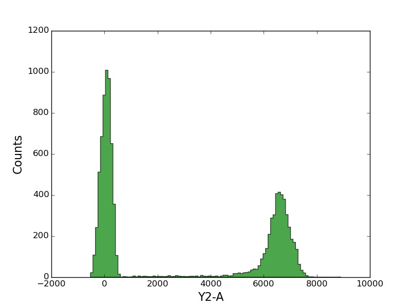
In [21]: figure();

In [22]: tsample.plot('Y2-A', bins=100);

In [23]: figure();

In [24]: grid(True)

In [25]: tsample.plot('Y2-A', color='green', alpha=0.7, bins=100);
If you provide the plot function with the names of two channels, you’ll get a 2d histogram.
In [26]: figure();

In [27]: tsample.plot(['B1-A', 'Y2-A']);
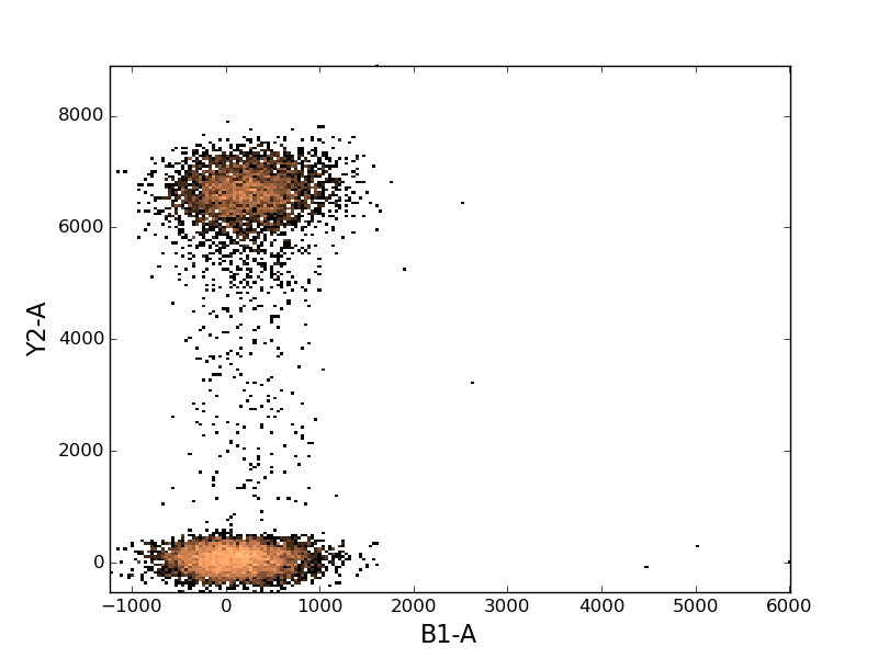
As with 1d histograms, the plot function accepts all the same arguments as does the matplotlib histogram function.
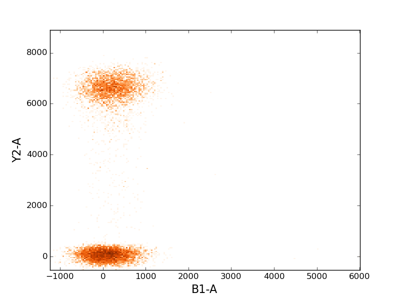
In [28]: figure();

In [29]: tsample.plot(['B1-A', 'Y2-A'], cmap=cm.Oranges, colorbar=False);
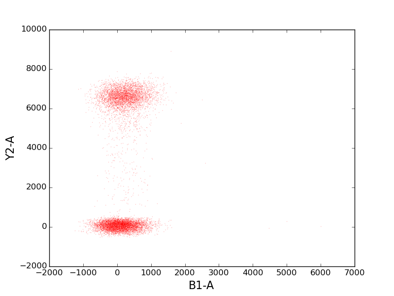
To create a scatter plot, provide the argument kind='scatter to the plot command.
This makes the plot function behave like the matplotlib scatter function (and accept all the same arguments).
In [30]: figure();

In [31]: tsample.plot(['B1-A', 'Y2-A'], kind='scatter', color='red', s=1, alpha=0.3);
See the API for a list of available gates.
Let’s import a few of those gates.
In [32]: from FlowCytometryTools import ThresholdGate, PolyGate
To create a gate you need to provide the following information:
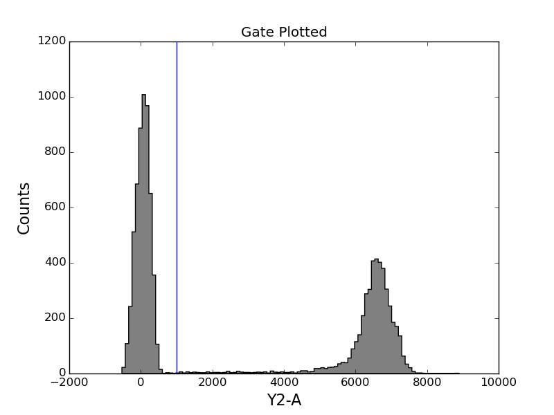
Let’s create a ThresholdGate that passes events with a Y2-A (RFP) value above the 1000.0.
In [33]: y2_gate = ThresholdGate(1000.0, 'Y2-A', region='above')
While we’re at it, here’s another gate for events with a B1-A value (CFP) above 2000.0.
In [34]: b1_gate = ThresholdGate(2000.0, 'B1-A', region='above')
You can launch the GUI for creating the gates, by calling the view_interactively() method of an FCMeasurement instance.
>>> tsample.view_interactively()
Warning
wxpython must be installed in order to use the GUI. (It may already be installed, so just try it out.)
Please note that there’s no way to apply transformations through the GUI, so view samples through the view_interactively method. (Don’t load new FCS files directly from the GUI, if you need those files transformed.)
In [35]: figure();

In [36]: tsample.plot('Y2-A', gates=[y2_gate], bins=100);

In [37]: title('Gate Plotted');
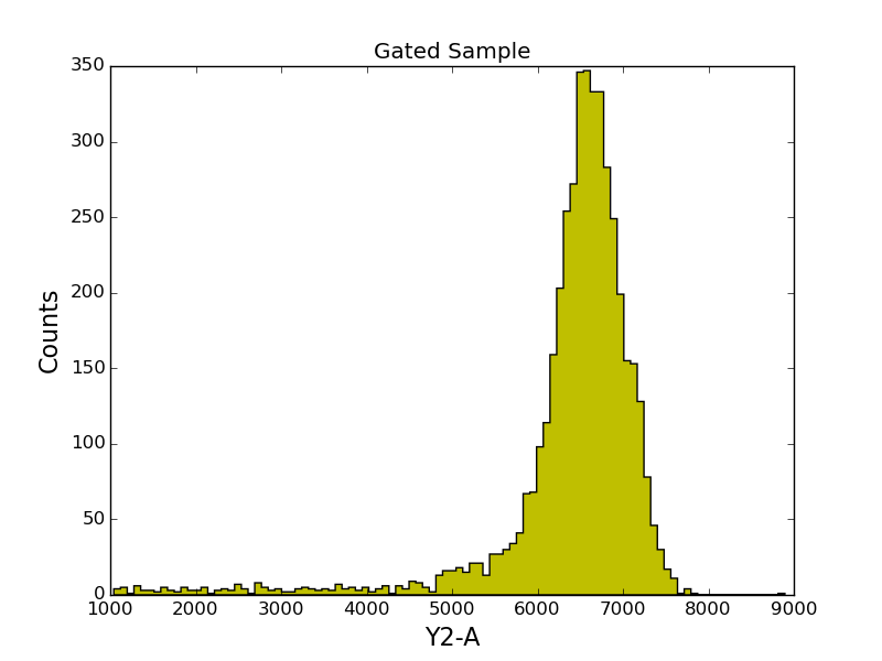
In [38]: gated_sample = tsample.gate(y2_gate)

In [39]: print gated_sample.get_data().shape[0]
4433
The gated_sample is also an instance of FCMeasurement, so it supports the same routines as does the ungated sample. For example, we can plot it:
In [40]: figure();

In [41]: gated_sample.plot('Y2-A', color='y', bins=100);

In [42]: title('Gated Sample');
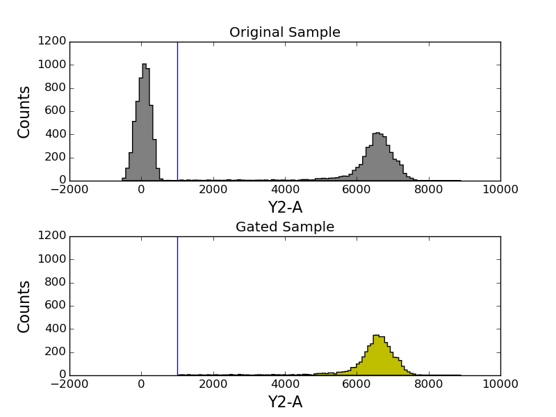
Let’s compare the gated and ungated side by side.
In [43]: figure();

In [44]: subplots_adjust(hspace=0.4)

In [45]: ax1 = subplot(211);

In [46]: tsample.plot('Y2-A', color='gray', bins=100, gates=[y2_gate]);

In [47]: title('Original Sample');

In [48]: ax2 = subplot(212, sharey=ax1, sharex=ax1);

In [49]: gated_sample.plot('Y2-A', color='y', bins=100, gates=[y2_gate]);

In [50]: title('Gated Sample');
Gates can be inverted and combined together. See FlowCytometryTools.core.gates.CompositeGate.
For high-throughput analysis of flow cytometery data, loading single FCS files is silly.
Instead, we provided you with the awesome FCPlate class (also called FCOrderedCollection).
The code below loads two FCS samples and shows two different methods of placing them on a plate container.
In [51]: from FlowCytometryTools import FCPlate

In [52]: sample1 = FCMeasurement('B1', datafile=datafile);

In [53]: sample2 = FCMeasurement('D2', datafile=datafile);

# Use the samples ID as their position on a plate:
In [54]: plate1 = FCPlate('demo plate', [sample1, sample2], 'name', shape=(4, 3))

In [55]: print plate1
ID:
demo plate

Data:
                      1                     2 3
A
B  <FCMeasurement 'B1'>
C
D                        <FCMeasurement 'D2'>

# Uses the dictionary key to map the position
In [56]: plate2 = FCPlate('demo plate', {'C1' : sample1, 'C2' : sample2}, 'name', shape=(4, 3))

In [57]: print plate2
ID:
demo plate

Data:
                      1                     2 3
A
B
C  <FCMeasurement 'B1'>  <FCMeasurement 'D2'>
D
Note
The method below should be simpler for 99% of the users to use (much less code!!), so keep on reading. :)
What we’d like to do is to construct a flow cytometry plate object by loading all the ‘*.fcs’ files in a directory.
To do that, FCPlate needs to know where on the plate each file belongs; i.e., we need to tell it that the file ‘My_awesome_data_Well_C9.fcs’ corresponds to well ‘C9’, which corresponds to the third row and the ninth column on the plate.
The process by which the filename is mapped to a position on the plate is the following:
Here’s a summary table that’ll help you decide what to do (depending on your file name format):
| File Name Format | parser | Comments |
|---|---|---|
| ‘[whatever]_Well_C9_[blah].fcs’ | ‘name’ | |
| ‘[blah]_someothertagC9_[blah].fcs’ | ‘name’ | But to use must modify ID_kwargs (see API) for details |
| ‘[whatever].025.fcs’ | ‘number’ | 001 -> A1, 002 -> B1, ... etc. i.e., advances by row first |
| Some other naming format | dict | dict with keys = filenames, values = positions |
| Some other naming format | function | Provide a function that accepts a filename and returns a position (e.g., ‘C9’) |
For the analysis below, we’ll be using the ‘name’ parser since our files match that convention. OK. Let’s try it out:
In [58]: from FlowCytometryTools import FCPlate

In [59]: plate = FCPlate.from_dir(ID='Demo Plate', path=datadir, parser='name')

In [60]: plate = plate.transform('hlog', channels=['Y2-A', 'B1-A'])
Let’s see what data got loaded.
In [61]: print plate
ID:
Demo Plate

Data:
  1  2                     3                     4  5                     6   \
A        <FCMeasurement 'A3'>  <FCMeasurement 'A4'>     <FCMeasurement 'A6'>
B        <FCMeasurement 'B3'>  <FCMeasurement 'B4'>
C
D
E
F
G
H

                     7  8  9  10 11 12
A  <FCMeasurement 'A7'>
B
C  <FCMeasurement 'C7'>
D
E
F
G
H
And just to confirm, let’s look at the naming of our files to see that parser='name' should indeed work.
In [62]: import os

In [63]: print os.path.basename(plate['A3'].datafile)
RFP_Well_A3.fcs
This plate contains many empty rows and columns. The method FCPlate.dropna() allow us to drop empty rows and columns for convenience:
In [64]: plate = plate.dropna()

In [65]: print plate
ID:
Demo Plate

Data:
                      3                     4                     6  \
A  <FCMeasurement 'A3'>  <FCMeasurement 'A4'>  <FCMeasurement 'A6'>
B  <FCMeasurement 'B3'>  <FCMeasurement 'B4'>
C

                      7
A  <FCMeasurement 'A7'>
B
C  <FCMeasurement 'C7'>
Please import matplotlib’s plotting functions if you haven’t yet...
In [66]: from pylab import *
For more information see FCPlate.plot().
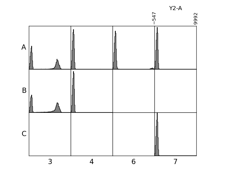
In [67]: figure();

In [68]: plate.plot('Y2-A', bins=100);
In [69]: figure();
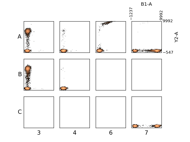
In [70]: plate.plot(('B1-A', 'Y2-A'), bins=100, wspace=0.2, hspace=0.2);
FCPlate supports indexing to make it easier to work with single wells.
In [71]: figure();

In [72]: print plate['A3']
<FCMeasurement 'A3'>

In [73]: plate['A3'].plot('Y2-A', bins=100);

Use the counts method to count total number of events.
In [74]: total_counts = plate.counts()

In [75]: print total_counts
       3      4      6      7
A  10000  10000  10000  10000
B  10000  10000    NaN    NaN
C    NaN    NaN    NaN  10000
Let’s count the number of events that pass a certain gate:
In [76]: y2_counts = plate.gate(y2_gate).counts()

In [77]: print y2_counts
      3   4    6   7
A  4433  50  420   6
B  5496   7  NaN NaN
C   NaN NaN  NaN   0
What about the events that land outside the y2_gate?
In [78]: outside_of_y2_counts = plate.gate(~y2_gate).counts()

In [79]: print outside_of_y2_counts
      3     4     6      7
A  5567  9950  9580   9994
B  4504  9993   NaN    NaN
C   NaN   NaN   NaN  10000
To learn how to do more complex calculations, let’s start by writing our own counting function. At the end of this, we better get the same result as was produced using the counts method above.
Here’s the function:
In [80]: def count_events(well):
   ....:     """ Counts the number of events inside of a well. """
   ....:     data = well.get_data()
   ....:     count = data.shape[0]
   ....:     return count
   ....:
Let’s check that it works on a single well.
In [81]: print count_events(plate['A3'])
10000
Now, to use it in a calculation we need to feed it to the apply method. Like this:
In [82]: print plate['A3'].apply(count_events)
10000
The apply method is a functional, which is just a fancy way of saying that it accepts functions as inputs. If you’ve got a function that can operate on a well (like the function count_events), you can feed it into the apply method. Check the API for the apply method for more details.
Anyway, the apply method is particularly useful because it works on plates.
In [83]: total_counts_using_our_function = plate.apply(count_events)

In [84]: print type(total_counts_using_our_function)
<class 'pandas.core.frame.DataFrame'>

In [85]: print total_counts_using_our_function
       3      4      6      7
A  10000  10000  10000  10000
B  10000  10000    NaN    NaN
C    NaN    NaN    NaN  10000
Holy Rabbit!
First, for wells without data, a nan was produced. Second, the output that was returned is a DataFrame.
Also, as you can see the total counts we computed (total_counts_using_our_function) agrees with the counts computed using the counts methods in the previous example.
Now, let’s apply a gate and count again.
In [86]: print plate.gate(y2_gate).apply(count_events)
      3   4    6   7
A  4433  50  420   6
B  5496   7  NaN NaN
C   NaN NaN  NaN   0
Ready for some more baking?
Let’s calculate the median Y2-A fluorescence.
In [87]: def calculate_median_rfp(well):
   ....:     """ Calculates the median on the RFP channel. """
   ....:     data = well.get_data()
   ....:     return data['Y2-A'].median()
   ....:
The median rfp fluorescence for all events in well ‘A3’.
In [88]: print calculate_median_rfp(plate['A3'])
303.091125488
The median rfp fluorescence for all events in the plate is:
In [89]: print plate.apply(calculate_median_rfp)
             3           4           6           7
A   303.091125  105.875381  136.326202  104.436157
B  4701.629395  126.765717         NaN         NaN
C          NaN         NaN         NaN   97.277603
The median rfp fluorescence for all events that pass the y2_gate is:
In [90]: print plate.gate(y2_gate).apply(calculate_median_rfp)
             3            4            6            7
A  6573.452148  6240.961426  9346.646484  9294.400391
B  6544.949219  6413.048340          NaN          NaN
C          NaN          NaN          NaN          NaN