Loading a single FCS file¶

To get cracking, we need some flow cytometry data (i.e., .fcs files).

A few sample flow cytometry data files have been bundled with this python package.

To locate these FCS files, enter the following:

In [1]: import os, FlowCytometryTools;
In [1]: datadir = os.path.join(FlowCytometryTools.__path__[0], 'tests', 'data', 'Plate01');
In [1]: datafile = os.path.join(datadir, 'RFP_Well_A3.fcs');

Alternatively, to analyze your own data, simply set the datafile variable to the path of your .fcs file. (e.g., datafile=r'C:\data\my_very_awesome_data.fcs').

If datadir and datafile have been defined, we can proceed to load the data:

In [1]: from pylab import * # Loads functions used for plotting

# Loading the FCS data
In [2]: from FlowCytometryTools import FCMeasurement

In [3]: sample = FCMeasurement(ID='Test Plate', datafile=datafile)

Windows Users

Windows uses the backslash character (\) for paths. However, the backslash character is a special character in python that is used for formatting strings. In order to specify paths correctly, you must precede the path with the character r.

Good: datafile=r'C:\data\my_very_awesome_data.fcs'

Bad: datafile='C:\data\my_very_awesome_data.fcs'

MacOS/Linux Users

Your system uses the forward slash (/), which is a regular character, so there won’t be any problems.

Channel Names¶

Want to know which channels were measured? No problem.

In [4]: print sample.channel_names
('HDR-T', 'FSC-A', 'FSC-H', 'FSC-W', 'SSC-A', 'SSC-H', 'SSC-W', 'V2-A', 'V2-H', 'V2-W', 'Y2-A', 'Y2-H', 'Y2-W', 'B1-A', 'B1-H', 'B1-W')

Hint

Full information about the channels is available in sample.channels.

Meta data¶

There’s loads of useful information inside FCS files. If you’re curious take a look at sample.meta.

In [5]: print type(sample.meta)
<type 'dict'>

In [6]: print sample.meta.keys()
['$ETIM', '$ENDDATA', '$BYTEORD', '$SRC', '_channels_', '$SYS', '$PAR', '$ENDANALYSIS', '$CYT', '__header__', '$BTIM', '$OP', '$BEGINANALYSIS', '$BEGINDATA', '$ENDSTEXT', '$CYTSN', '$DATE', '$MODE', '$FIL', '$BEGINSTEXT', '$NEXTDATA', '$CELLS', '$TOT', '_channel_names_', '$DATATYPE']

The meaning of the fields in sample.meta is explained in the FCS format specifications.

Transformations¶

The presence of both very dim and very bright cell populations in flow cytometry data can make it difficult to simultaneously visualize both populations on the same plot. To address this problem, flow cytometry analysis programs typically apply a transformation to the data to make it easy to visualize and interpret properly.

Rather than having this transformation applied automatically and without your knowledge, this package provides a few of the common transformations (e.g., hlog, tlog), but ultimately leaves it up to you to decide how to manipulate your data.

As an example, let’s apply the ‘hlog’ transformation to the Y2-A, B1-A and V2-A channels, and save the transformed sample in tsample.

In [7]: tsample = sample.transform('hlog', channels=['Y2-A', 'B1-A', 'V2-A'])

Note that throughout the rest of the tutorial we’ll always be working with hlog-transformed data.

Note

For more details see the API documentation section.

Also, you can read more about transformations here:

Bagwell. Cytometry Part A, 2005.
Parks, Roederer, and Moore. Cytometry Part A, 2006.
Trotter, Joseph. In Current Protocols in Cytometry. John Wiley & Sons, Inc., 2001.

Plotting¶

1d histograms¶

Let’s start with 1d histograms.

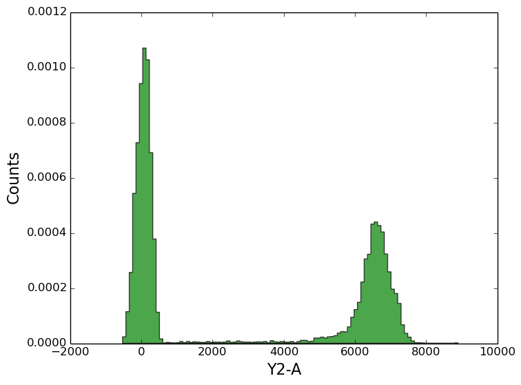
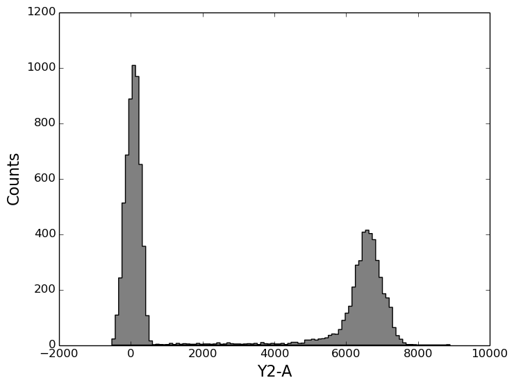
In [8]: figure();
In [8]: tsample.plot('Y2-A', bins=100);

The plot function accepts all the same arguments as does the matplotlib histogram function.

In [8]: figure();
In [8]: tsample.plot('Y2-A', bins=100, alpha=0.7, color='green', normed=1);

2d histograms¶

If you feed the plot function with the names of two channels, you’ll get a 2d histogram.

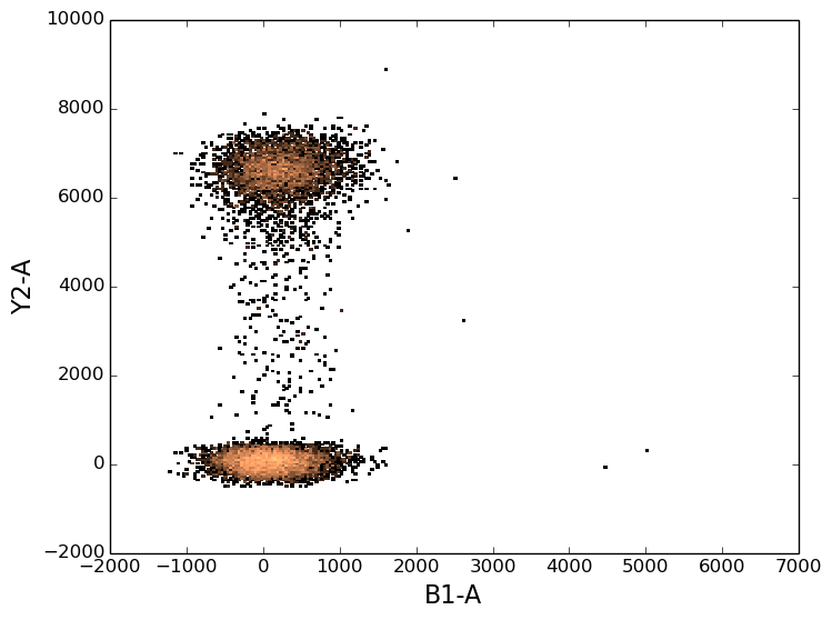
In [8]: figure();
In [8]: tsample.plot(['B1-A', 'Y2-A']);

As with 1d histograms, the plot function accepts all the same arguments as does the matplotlib histogram function.

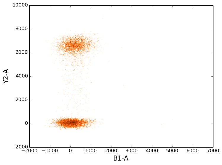
In [8]: figure();
In [8]: tsample.plot(['B1-A', 'Y2-A'], cmap=cm.Oranges, colorbar=False);

2d scatter plots¶

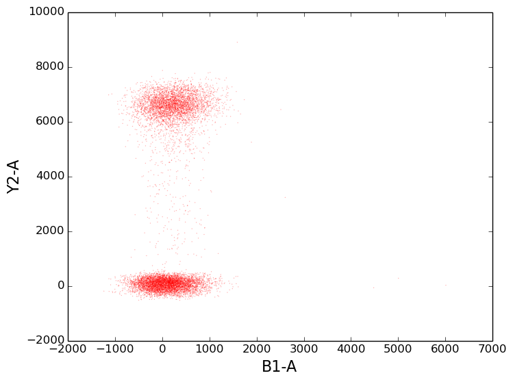
To create a scatter plot, provide the argument kind='scatter to the plot command.

This makes the plot function behave like the matplotlib scatter function (and accept all the same arguments).

In [8]: figure();
In [8]: tsample.plot(['B1-A', 'Y2-A'], kind='scatter', color='red', s=1, alpha=0.3);

Calculations¶

In [8]: data = tsample.get_data()

In [9]: print data
<class 'pandas.core.frame.DataFrame'>
Int64Index: 10000 entries, 0 to 9999
Data columns (total 16 columns):
HDR-T    10000  non-null values
FSC-A    10000  non-null values
FSC-H    10000  non-null values
FSC-W    10000  non-null values
SSC-A    10000  non-null values
SSC-H    10000  non-null values
SSC-W    10000  non-null values
V2-A     10000  non-null values
V2-H     10000  non-null values
V2-W     10000  non-null values
Y2-A     10000  non-null values
Y2-H     10000  non-null values
Y2-W     10000  non-null values
B1-A     10000  non-null values
B1-H     10000  non-null values
B1-W     10000  non-null values
dtypes: float32(16)

That’s right. Your data is a pandas DataFrame, which means that you’ve got the entire power of pandas at your fingertips!

In [10]: print data['Y2-A'].describe()
count    10000.000000
mean      2871.126400
std       3210.111110
min       -528.319885
25%         39.917786
50%        303.091125
75%       6510.390747
max       8895.525391
dtype: float64

Want to know how many events are in the data?

In [11]: print data.shape[0]
10000

Want to calculate the median fluorescence level measured on the Y2-A channel?

In [12]: print data['Y2-A'].median()
303.091125488

Gating¶

First, we need to load the gates from the library.

In [13]: from FlowCytometryTools import ThresholdGate, PolyGate

Creating Gates¶

Programmatically¶

To create a gate you need to provide the following information:

set(s) of coordinates
name(s) of channel(s)
region

For example, here’s a gate that passes events with a Y2-A (RFP) value above the 1000.0.

In [14]: y2_gate = ThresholdGate(1000.0, 'Y2-A', region='above')

While we’re at it, here’s another gate for events with a B1-A value (CFP) above 2000.0.

In [15]: b1_gate = ThresholdGate(2000.0, 'B1-A', region='above')

Using the GUI¶

You can launch the GUI for creating the gates, by calling the view() method of an FCMeasurement instance.

tsample.view()

Warning

You have to install wxpython in order to use the GUI.

Also, keep in mind that the GUI is still in early stages. Expect bugs.

Plotting Gates¶

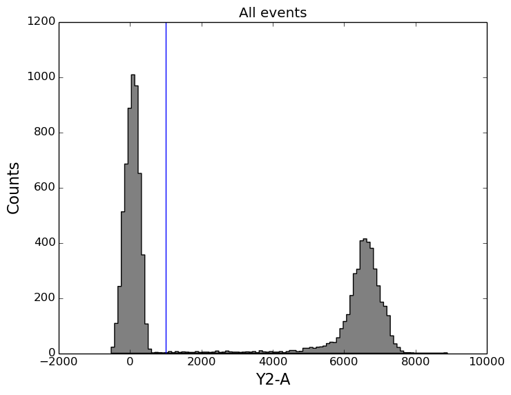
In [16]: figure();
In [16]: ax1 = subplot(111);
In [16]: tsample.plot('Y2-A', gates=[y2_gate], apply_gates=False, bins=100);
In [16]: title('All events');
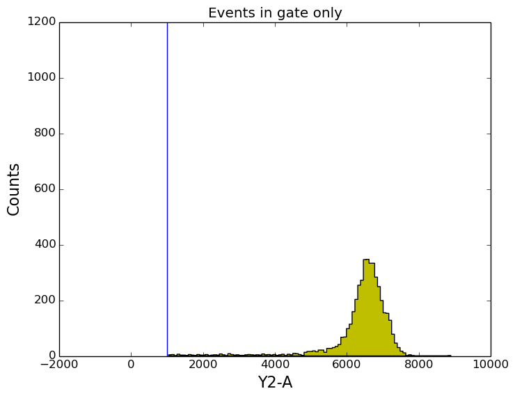
In [16]: figure();
In [16]: ax2 = subplot(111, sharey=ax1, sharex=ax1);
In [16]: tsample.plot('Y2-A', gates=[y2_gate], apply_gates=True, bins=100, color='y');
In [16]: title('Events in gate only');

Applying Gates¶

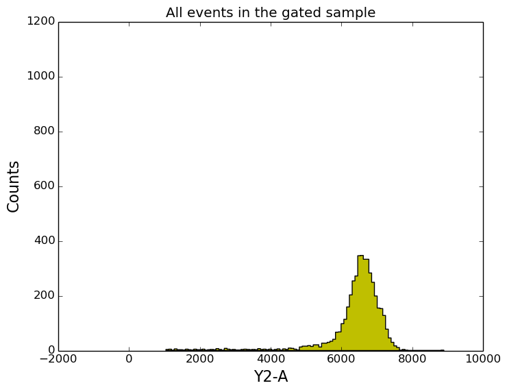
In [16]: gated_sample = tsample.gate(y2_gate)

In [17]: print gated_sample.get_data().shape[0]
4433

The gated_sample is also an FCMeasurement, so it supports the same routines as the ungated sample. For example, we can plot it:

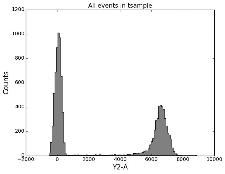
In [18]: figure();
In [18]: ax1 = subplot(111);
In [18]: tsample.plot('Y2-A', color='gray', bins=100);
In [18]: title('All events in tsample');
In [18]: figure();
In [18]: ax2 = subplot(111, sharey=ax1, sharex=ax1);
In [18]: gated_sample.plot('Y2-A', color='y', bins=100);
In [18]: title('All events in the gated sample');

Working with plates¶

For high-throughput analysis of flow cytometery data, loading single FCS files is silly.

Instead, we provided you with the awesome FCPlate class!

Loading Data¶

What we’d like to do is to construct a flow cytometry plate object by loading all the ‘*.fcs’ files in a directory.

To do that, FCPlate needs to know where on the plate each file belongs; i.e., we need to tell it that the file ‘My_awesome_data_Well_C9.fcs’ corresponds to well ‘C9’, which corresponds to the third row and the ninth column on the plate.

The process by which the filename is mapped to a position on the plate is the following:

The filename is fed into a parser which extracts a key from it. For example, given ‘My_awesome_data_Well_C9.fcs’, the parser returns ‘C9’
The key is fed into a position mapper which returns a matrix position. For example, given ‘C9’ the position_mapper should return (2, 8). The reason it’s (2, 8) rather than (3, 9) is because counting starts from 0 rather than 1. (So ‘A’ corresponds to 0.)

Here’s a summary table that’ll help you decide what to do (depending on your file name format):

File Name Format	parser	Comments
‘[whatever]_Well_C9_[blah].fcs’	‘name’
‘[blah]_someothertagC9_[blah].fcs’	‘name’	But to use must modify ID_kwargs (see API) for details
‘[whatever].025.fcs’	‘number’	001 -> A1, 002 -> B1, ... etc. i.e., advances by row first
Some other naming format	dict	dict with keys = filenames, values = positions
Some other naming format	function	Provide a function that accepts a filename and returns a position (e.g., ‘C9’)

For the analysis below, we’ll be using the ‘name’ parser since our files match that convention. OK. Let’s try it out!

In [18]: from FlowCytometryTools import FCPlate

In [19]: plate = FCPlate.from_dir(ID='Demo Plate', path=datadir, parser='name').transform('hlog', channels=['Y2-A', 'B1-A'])

Let’s see what data got loaded...

In [20]: print plate
ID:
Demo Plate
Data:
  1  2     3     4  5     6     7  8  9  10 11 12
A        'A3'  'A4'     'A6'  'A7'               
B        'B3'  'B4'                              
C                             'C7'               
D                                                
E                                                
F                                                
G                                                
H                                                

And just to confirm, let’s look at the naming of our files to see that parser='name' should indeed work.

In [21]: import os

In [22]: print os.path.basename(plate['A3'].datafile)
RFP_Well_A3.fcs

This plate contains many empty rows and columns, which may be dropped for convenience.

In [23]: plate = plate.dropna()

In [24]: print plate
ID:
Demo Plate
Data:
      3     4     6     7
A  'A3'  'A4'  'A6'  'A7'
B  'B3'  'B4'            
C                    'C7'

Plotting¶

In [25]: figure();
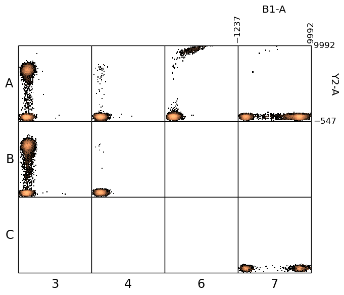
In [25]: plate.plot('Y2-A', bins=100);

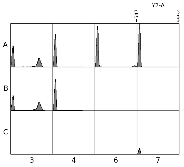
In [25]: figure();
In [25]: plate.plot(('B1-A', 'Y2-A'), bins=100);

Accessing Single Wells¶

FCPlate supports indexing to make it easier to work with single wells.

In [25]: figure();
In [25]: print plate['A3']
'A3'

In [26]: plate['A3'].plot('Y2-A', bins=100);

Examples¶

Counting using the counts method¶

Use the counts method to count total number of events.

In [26]: total_counts = plate.counts()

In [27]: print total_counts
       3      4      6      7
A  10000  10000  10000  10000
B  10000  10000    NaN    NaN
C    NaN    NaN    NaN  10000

Let’s count the number of events that pass a certain gate:

In [28]: y2_counts = plate.gate(y2_gate).counts()

In [29]: print y2_counts
      3   4    6   7
A  4433  50  420   6
B  5496   7  NaN NaN
C   NaN NaN  NaN   0

What about the events that land outside the y2_gate?

In [30]: outside_of_y2_counts = plate.gate(~y2_gate).counts()

In [31]: print outside_of_y2_counts
      3     4     6      7
A  5567  9950  9580   9994
B  4504  9993   NaN    NaN
C   NaN   NaN   NaN  10000

Counting on our own¶

To learn how to do more complex calculations, let’s start by writing our own counting function. At the end of this, we better get the same result as was produced using the counts method above.

Here’s the function:

In [32]: def count_events(well):
   ....:     """ Counts the number of events inside of a well. """
   ....:     data = well.get_data()
   ....:     count = data.shape[0]
   ....:     return count
   ....:

Let’s check that it works on a single well.

In [33]: print count_events(plate['A3'])
10000

Now, to use it in a calculation we need to feed it to the apply method. Like this:

In [34]: print plate['A3'].apply(count_events)
10000

The apply method is a functional, which is just a fancy way of saying that it accepts functions as inputs. If you’ve got a function that can operate on a well (like the function count_events), you can feed it into the apply method. Check the API for the apply method for more details.

Anyway, the apply method is particularly useful because it works on plates.

In [35]: total_counts_using_our_function = plate.apply(count_events)

In [36]: print type(total_counts_using_our_function)
<class 'pandas.core.frame.DataFrame'>

In [37]: print total_counts_using_our_function
       3      4      6      7
A  10000  10000  10000  10000
B  10000  10000    NaN    NaN
C    NaN    NaN    NaN  10000

Holy Rabbit! That was smokin’ hot output!

First, for wells without data, a nan was produced. Second, the output that was returned is a DataFrame.

Also, as you can see the total counts we computed (total_counts_using_our_function) agrees with the counts computed using the counts methods in the previous example.

Now, let’s apply a gate and count again.

In [38]: print plate.gate(y2_gate).apply(count_events)
      3   4    6   7
A  4433  50  420   6
B  5496   7  NaN NaN
C   NaN NaN  NaN   0

Calculating median fluorescence¶

Ready for some more baking?

Let’s calculate the median Y2-A fluorescence.

In [39]: def calculate_median_rfp(well):
   ....:     """ Calculates the median on the RFP channel. """
   ....:     data = well.get_data()
   ....:     return data['Y2-A'].median()
   ....:

The median rfp fluorescence for all events in well ‘A3’.

In [40]: print calculate_median_rfp(plate['A3'])
303.091125488

The median rfp fluorescence for all events in the plate is:

In [41]: print plate.apply(calculate_median_rfp)
             3           4           6           7
A   303.091125  105.875378  136.326202  104.436157
B  4701.629395  126.765717         NaN         NaN
C          NaN         NaN         NaN   97.277603

The median rfp fluorescence for all events that pass the y2_gate is:

In [42]: print plate.gate(y2_gate).apply(calculate_median_rfp)
             3            4            6            7
A  6573.452148  6240.961426  9346.645996  9294.400391
B  6544.948975  6413.048340          NaN          NaN
C          NaN          NaN          NaN          NaN